

Probing the SynthID-text deployment on Gemini APIs
Thibaud Gloaguen, Robin Staab, Kristian Minchev, Martin Vechev
October 21, 2026
SynthID-Text is the first major publicized large-scale deployment of an LLM watermarking algorithm, announced in 2024. It was originally deployed in the Gemini app, and following the requirements of the EU AI Act is allegedly deployed in the API. While Google released an open-source implementation of SynthID-Text, they have not discussed how they deploy their watermark in practice. In this blog post, using our ICLR 2025 work, we answer the following questions:
- Do all Gemini models share the same watermark?
- What are the hyperparameters used by the deployed SynthID-Text?
- Is the (hidden) thinking trace watermarked?
Answering those questions has important practical implications. With the watermark hyperparameters, attackers can then mount more sophisticated watermark stealing attacks that allow them to either remove or spoof the watermark. Furthermore, knowing that lite models use the same watermark as larger models enables attackers to attack the SynthID watermark at a much lower cost. Lastly, knowing whether the thinking trace is watermarked has significant implications for the research community. In particular, recent works (ReasonMark, Marking the Wrong Symptoms: Evaluating LLM Watermarks in Medical Texts) have been discussing whether the thinking trace should be watermarked and how watermarking the thinking trace impacts reasoning accuracy.
How does text watermarking work?
The idea behind most LLM watermarks, including SynthID-Text, is to change the probabilities of the next tokens to leave a detectable pattern in the generated text. Let’s start with a small example.
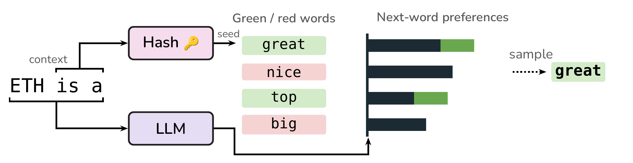
Illustration of the Red-Green watermarking algorithm. Given a partial sentence, the LLM outputs a probability distribution over the next token. The watermark uses the previously generated token as a seed to partition the vocabulary into red and green tokens. It then increases the probability of green tokens. Thus, a watermarked text has more green tokens than a non-watermarked one.
The LLM is generating the following text: “ETH is a” and needs to choose the next word. Let’s assume that the LLM gives a probability of 1/2 to “great” and 1/2 to “nice”. Without a watermark, the sampling algorithm would simply choose either word with probability 1/2. A simple watermark could increase the probability of “great” to 3/4 (green word) and decrease that of “nice” to 1/4 (red word). Here the color is chosen deterministically by the watermark. Both words are still possible, but “great” is now chosen more often! Repeating this kind of transformation throughout the text leaves a statistical pattern: the generated text contains more of the green words favored by the watermark than we would otherwise expect.
SynthID-Text uses a more complex transformation than this simple probability shift, designed to not alter the quality of the generated text. But the underlying idea remains the same: change the probabilities deterministically so that the text carries a detectable statistical pattern.
How do we decide which tokens to favor? The deterministic choice should look random, but the watermark detector needs to be able to reproduce it. To achieve this, the watermark combines a secret key with a few preceding tokens, called the watermark’s context, to compute a seed. This seed determines which tokens are favored: the same key and context give the same choices, while a different context can favor different tokens. A detector with the key can reconstruct these choices from the text and check whether unusually many favored tokens were generated. This reproducibility across queries is also the property our black-box tests exploit.
Black-Box Detection of Language Model Watermarks
In “Black-Box Detection of Language Model Watermarks”, we introduced several statistical tests that allow us to detect, from text responses alone, whether an API is watermarked or not. We have now updated our method to be more resilient to modern LLM scenarios (e.g., thinking models).
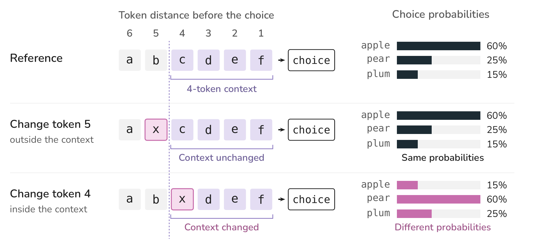
Illustration of context-size probing. Changing a token outside the four-token watermark context preserves the choice probabilities, while changing one inside it changes them.
In our original work, we asked the LLM to choose a random word and tested whether its word preferences depended strongly on the preceding tokens. To infer the watermark context length, we require replies of the form \(t_{n}\dots t_{1} \text{choice}\), where \(t_{i}\) is the token \(i\) positions before the chosen word. For each position \(i\), we vary \(t_{i}\) while keeping all other preceding tokens fixed, then compare the choice probabilities across repeated replies.
If \(i\) is smaller than or equal to the watermark context length (e.g., \(i = 4\) in the example above, with a context length of 4), changing \(t_{i}\) changes the watermark context and therefore which tokens the watermark favors. We thus expect the choice probabilities to change. If \(i\) is greater than the watermark context length (e.g., \(i = 5\) in the example above), changing \(t_{i}\) leaves the watermark context unchanged, so the watermark should continue to favor the same tokens.
Autoresearch to update our method
The original method presented above faces several issues when used in practice, e.g., thinking models may decide the choice of the words in their thinking trace without the intended context.
User: Finish the sentence: "I bought 2222" using a word from the list [bananas, strawberries, apples, pears].

Model: <think>I am asked to finish the sentence with a word from the list. I will use the word bananas. Thus my final answer is: 'I bought 2222 bananas'.</think>
I bought 2222 bananas.
In this example, the word bananas was chosen by the model in the thinking trace: there is no influence due to the context 2222 and thus our test would have failed.
To update our method, we let auto-research agents figure out how to overcome this issue. Specifically, we gave an Opus 5.5 agent access to 3 black-box APIs (from its perspective) with only 1 of them watermarked. The agent was tasked with figuring out which one is watermarked. It also had access to a local GPU for conducting its experiments. After about 24 hours of research, it came up with an improvement to our method!
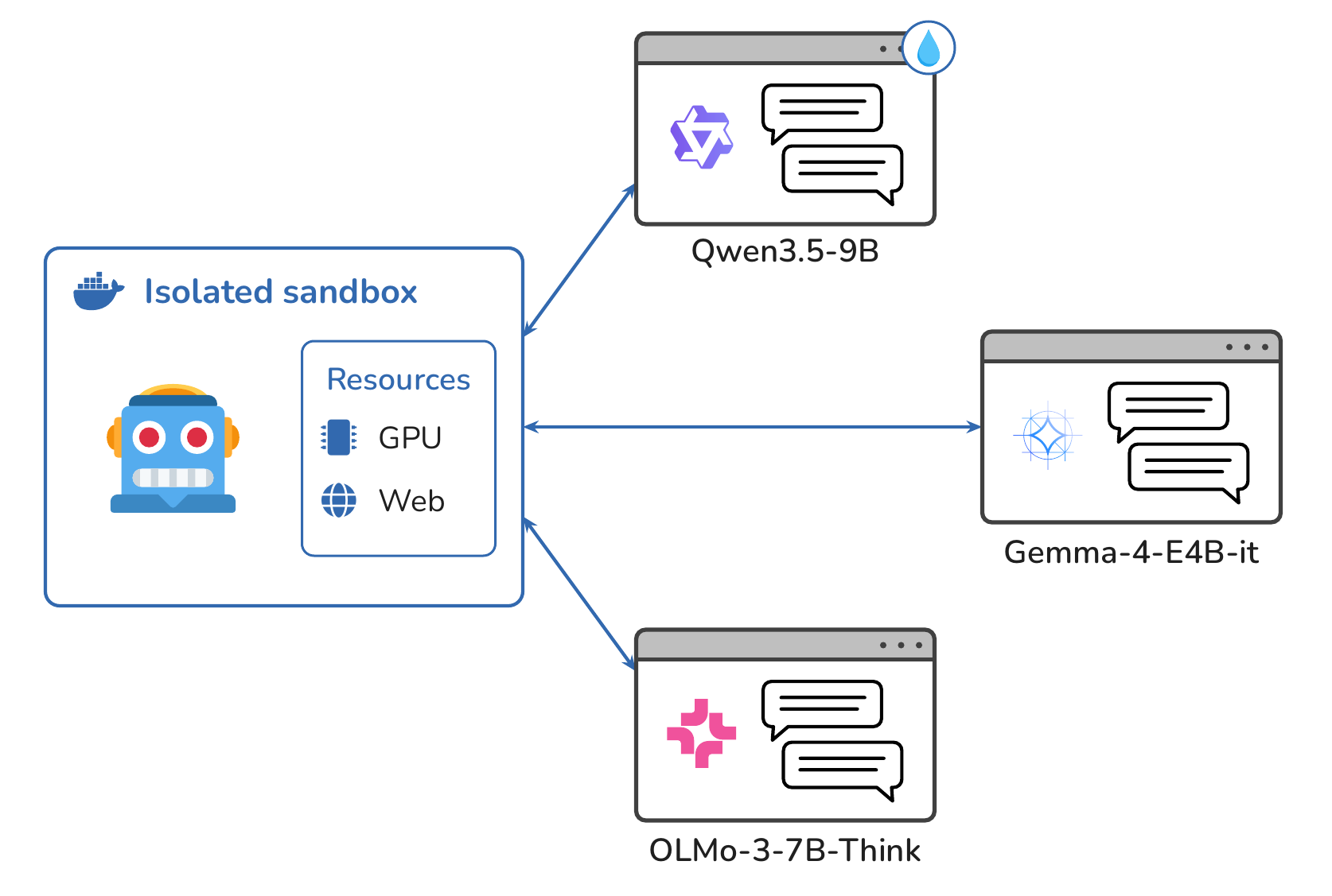
Illustration of our autoresearch setup. An Opus5.5 agent is running in an isolated sandbox and has access to 3 black-box APIs, one of them being watermarked. It is tasked to design a test to infer which one is watermarked.
The three black-box APIs served Qwen3.5-9B, Gemma-4-E4B-it, and Olmo-3-7B-Think, with their identities hidden from the agent. For local experiments, the agent had access to LiquidAI’s LFM2.5-2.6B on an NVIDIA RTX PRO 6000 GPU (96 GB). Downloading any additional model weights, from Hugging Face or elsewhere, was forbidden, preventing direct comparisons between the APIs and local copies of the same models.
The updated method still tests whether word preferences depend on the preceding tokens. To keep those tokens next to the chosen word even during thinking, we ask the model to write a story with a code at the start of each sentence:
Answer immediately without deliberation. Write a story about a lighthouse keeper in exactly 20 sentences, one sentence per line. Each line must begin with the given code copied exactly (single letters separated by single spaces), then a space, then the sentence. Use these codes in this order, one per line:
r o o g o p d y
j d u d c o p d
e y h u k t v r
[17 more codes]
Output only the 20 lines.
Here, each code gives the sequence \(t_n\dots t_1\) before the opening word. We let the model choose any opening word, giving it more entropy than a fixed list. The eight letters in this example are a choice we make when designing the prompt. Below, we use sixteen letters to probe contexts longer than four tokens. The code length and the number of sentences are chosen separately. A typical reply would be
<think>I'll start by drafting the sentences. I'll need to create a narrative arc,
building a sense of place and atmosphere.

r o o g o p d y Silas climbed the spiral iron staircase as the sun began to sink below the jagged horizon.
j d u d c o p d The brass lantern housing gleamed under his weathered, calloused hands.
e y h u k t v r Outside, a brisk northern wind howled against the thick granite tower walls.
[...]</think>

r o o g o p d y Silas climbed the spiral iron staircase as the sun began to sink below the jagged horizon.
j d u d c o p d The brass lantern housing gleamed under his weathered, calloused hands.
e y h u k t v r Outside, a brisk northern wind howled against the thick granite tower walls.
[...]
In this example, the code immediately precedes the opening word when the model first drafts it in the thinking trace. If thinking is watermarked, the code can therefore influence the word choice. Copying this draft into the visible answer preserves that bias. With thinking disabled, the model chooses the word directly after the code in its visible answer. This lets us apply the same test in both settings.
To compare codes with different amounts of shared context, we construct 20 families before querying the model. Each family starts with one random 16-letter reference code. We create eight variants that share exactly 0, 1, 2, 3, 4, 6, 8, or 12 trailing letters with it. For each variant, we keep the suffix, change the letter immediately before it, and randomly draw the earlier letters, keeping the first letter fixed. We also add two controls that preserve the first 12 or 14 letters and change the last letter. Each family thus contains 11 codes, giving 220 codes in total. Keeping the first letter fixed helps control for models that use it to choose the first letter of the opening word.
For example, these shorter codes all share the last three letters t d f:
r a p t d f
r e s t d f
r z o t d f
We count shared trailing letters backwards from the code endings, stopping at the first difference. The first two codes above share exactly three trailing letters. The second and third share four.
For each tested model, we also verify that each letter corresponds exactly to one token (it would be possible for tokenizers to tokenize e.g.
a bin a single token). This lets us count the tokens immediately before the opening word from the letters in the code.
For each story, we randomly select one code from each family and shuffle their order. Each of the 20 lines uses one selected code. We repeat this with new stories and record each code together with the first word that follows it. The code pool stays fixed throughout the experiment. After collecting the replies, we use the same observations to analyze every tested suffix length.
For each code, we build a word-preference profile by comparing the observed word counts with the counts expected if word choice did not depend on the code. We use the 12 most frequent opening words and group the remaining words into an “other” category. A positive profile entry means that a word appears more often than expected, and a negative entry means that it appears less often. We scale each difference by the square root of its expected count.
Let’s work through a small example. Suppose we use five-letter codes and each sentence starts with “The”, “Silas” (a character’s name), or “Outside”. For example, r b c d y Silas climbed the stairs. gives us the code r b c d y followed by the word “Silas”. In one family, we have the reference r b c d y and two variants, r l x d y and r j k x y. For each story, we select one of these codes and record the word that follows it. The first variant shares two trailing letters with the reference, while the second shares only one.
Suppose we observe the reference 30 times: 12 followed by “The”, 9 by “Silas”, and 9 by “Outside”. Across all codes, the three words appear equally often, so we would expect 10 of each for this code. Its profile is therefore \((2,-1,-1)/\sqrt{10}\). If r l x d y gives the same counts, the two codes favor the same words. If r j k x y instead gives counts of 10, 13, and 7, it favors “Silas” and disfavors “Outside”. Repeating this comparison across families, we would look for word preferences that become similar once codes share two trailing tokens. This would suggest a two-token watermark context.
We then compare these profiles for codes sharing different numbers of trailing tokens. If the watermark uses a context of 4 tokens, codes sharing only their last 3 tokens generally produce different watermark seeds and therefore different word preferences. Once they share their last 4 tokens, their seeds match, and their preferences should become as similar as those observed with the same code. We therefore look for a sudden jump in similarity, followed by a plateau: the location of the jump reveals the watermark’s context size!
Precisely, we randomly split the collected replies into halves \(A\) and \(B\). Let \(N^A_{cw}\) count how often code \(c\) is followed by word \(w\) in half \(A\). Let \(n^A_c\) be the total count for code \(c\), \(n^A_w\) the total for word \(w\), and \(n^A\) the total number of observations. Under independence between codes and words, the expected count is \(E^A_{cw}=n^A_c n^A_w/n^A\). Define the standardized residual \(R^A_{cw}=(N^A_{cw}-E^A_{cw})/\sqrt{E^A_{cw}}\), and similarly for half \(B\). The similarity between any two codes \(c\) and \(d\) is
\[G_{cd}=\frac12\sum_w\left(R^A_{cw}R^B_{dw}+R^B_{cw}R^A_{dw}\right).\]Within each family, we average \(G_{cd}\) over distinct code pairs sharing exactly \(m\) trailing tokens. We then average equally across families to obtain \(S_m\). Pairs sharing no trailing tokens but a long prefix are kept as separate controls and excluded from \(S_0\). We also average over multiple random splits of the replies. A larger \(S_m\) means that these codes reproducibly favor and disfavor the same words.
Let \(S_0\) be the baseline for codes sharing no trailing tokens, and \(S_{\mathrm{same}}\) the average similarity of each code with itself across the two halves. For each suffix length \(m\), we define the alignment \(r_m=(S_m-S_0)/(S_{\mathrm{same}}-S_0)\). An alignment near 0 means that sharing \(m\) trailing tokens produces as little similarity as sharing none. An alignment near 1 means that these codes have word preferences as similar as those measured with the same code.
We give a worked example with two small families, three possible opening words, and detailed calculations.
Applying our method to all Gemini models
We apply our method to ten Gemini models using the same 20 families of 16-letter codes described above. We collect 2,000 stories per model, except for Gemini 2.5 Pro (1,200) and Gemini 3.7 Flash (1,990 retained). Each story provides up to 20 code–word observations, giving up to 40,000 observations per model, or about 182 per code. From these replies, we compute alignment at shared suffix lengths 1, 2, 3, 4, 6, 8, and 12, using length 0 as the baseline and identical codes for calibration. We disable thinking whenever the API allows it.
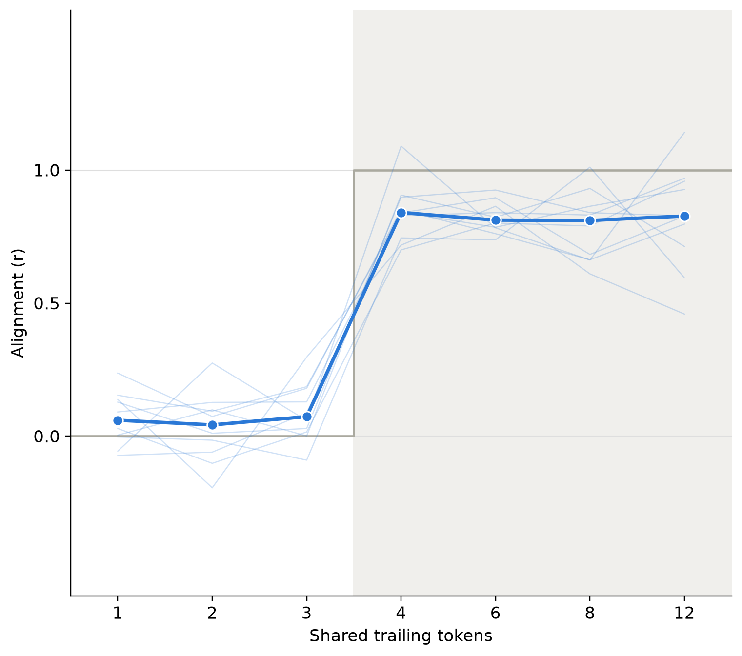
Within-model alignment for 10 Gemini models as a function of the number of shared trailing tokens. Faint blue curves show individual models and the thick blue curve shows their median. The jump at four shared tokens is consistent with a four-token watermark context across all evaluated models.
Our results show that, for codes sharing exactly 3 trailing tokens, we see no similar word preferences across codes on any model. However, for codes sharing 4 or more trailing tokens, we see on all models that different codes consistently lead to the same word preferences. This means that the watermark context size of all evaluated Gemini models is 4 tokens.
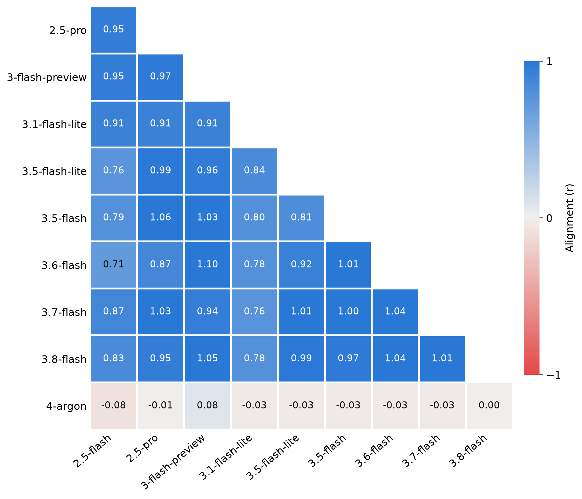
Alignment between the watermark biases of 10 Gemini models. All models except Gemini 4 Argon share the same context bias, consistent with a shared watermarking key. Gemini 4 Argon has no detectable alignment with those models and thus effectively has a different watermarking key.
Furthermore, if we look at the word preference across the nine models from Gemini 2.5 to 3.8, we find that for each shared set of trailing tokens, these models show the same word preference. This is consistent with those nine models sharing the exact same watermarking key. Gemini 4 Argon also has a four-token watermark context, but its biases do not align with those of the earlier models in any of the nine comparisons. This lack of alignment means that Argon effectively has a different watermarking key. This result is actually not surprising: the watermark is applied at the token level, and Gemini 4 uses a different tokenizer compared with previous models. This means that the watermark is also applied differently, similar to having a different key.
Detecting that the thinking trace is watermarked
A question in the watermark literature is whether model providers should watermark the thinking trace (ReasonMark, Marking the Wrong Symptoms: Evaluating LLM Watermarks in Medical Texts). With our probing, we find that Google decided to watermark the thinking traces of Gemini.
We realized the thinking trace of Gemini 3.8 Flash is watermarked quite inadvertently. On the Gemini 3.8 Flash API, you can enable/disable the thinking trace. We therefore ran the above experiment with thinking enabled and disabled.
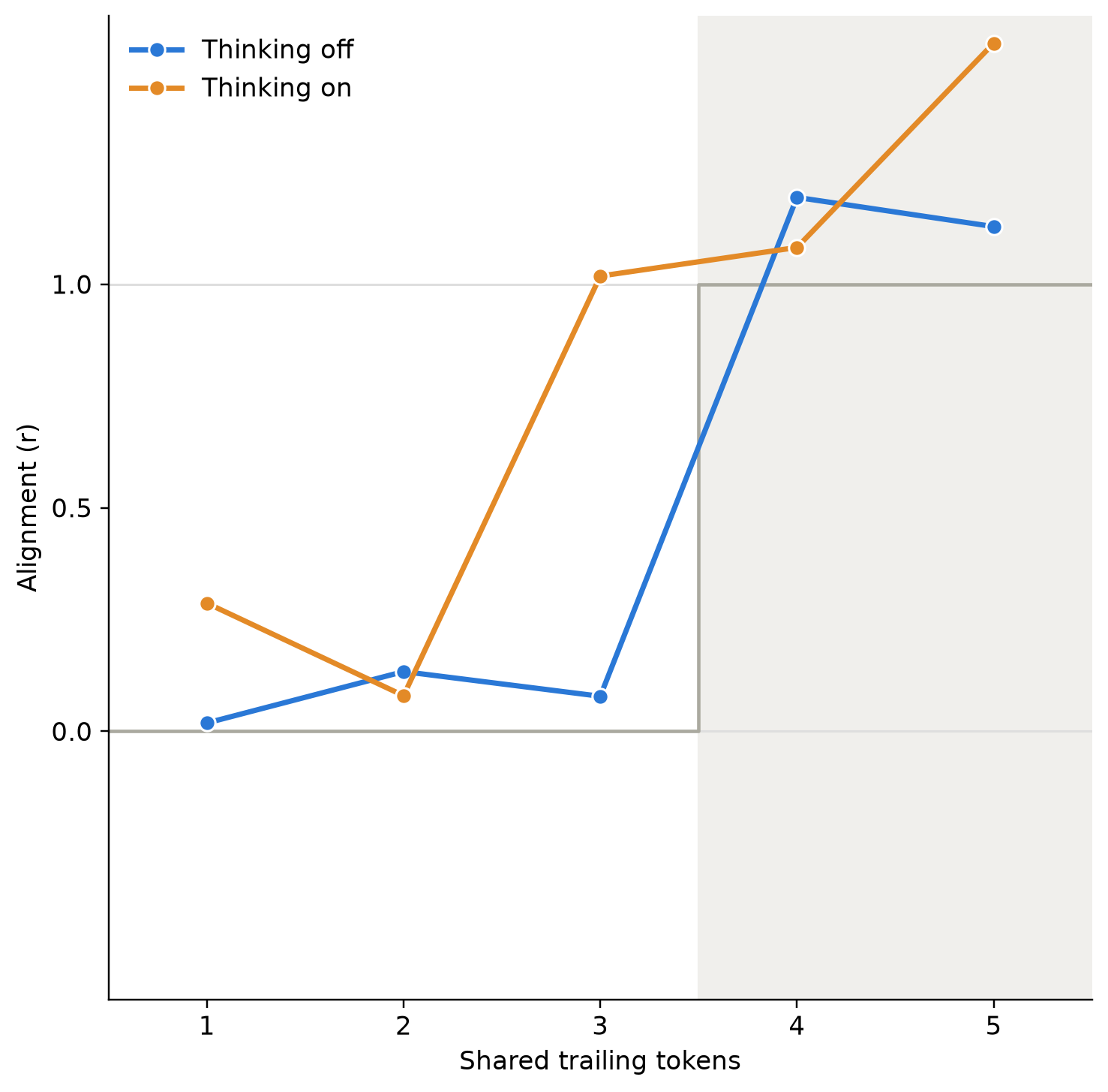
Alignment scores for Gemini 3.8 Flash without and with thinking depending on the number of shared trailing tokens in each code word. We see that the alignment jumps at 4 tokens without thinking and 3 with thinking.
As we can see in the figure, the jump in similarity appears at 3 tokens with thinking on (orange curve) whereas it appears at 4 tokens with thinking off (blue curve). This seems to suggest that the watermark context is not the same when thinking is on or off. But is it really?
Because of these unexpected results, we pushed our investigation further. The Gemini API allows us to obtain thinking summaries of the thinking trace. We therefore decided to look in detail at those summaries.
1.  `g e x q m j h r` High atop the jagged peaks of Mount Ashen, a solitary beast slumbered beneath centuries of frozen mist.
2.  `f r x t k b m o` His crimson scales shimmered like polished rubies caught in the pale morning sun.
3.  `h b x f o d d r` For a thousand years, the dragon had ignored the petty squabbles of the mortal realm below.
The summaries sometimes show a backtick between the code and the first word. If the model also inserts it when drafting the story in its hidden trace, the backtick takes up one token of the watermark context. A four-token context would then contain the last three tokens of the code and the backtick, explaining the jump at 3 shared tokens.
To test this explanation, we collected 500 additional stories with thinking disabled, using the same code pool and adding a closing backtick after every code. The resulting word preferences align with those measured with thinking enabled, supporting the explanation that the model chooses the words after a backtick during thinking and copies them into its visible answer. Thinking summaries are rewritten accounts of the hidden trace, so the controlled comparison provides stronger evidence than the summaries alone.
Why watermark the thinking trace?
We now know that Google decided to watermark the thinking trace of their model. In this part, we try to give sensible explanations for why this choice makes sense.
Intuitively, because the thinking trace is hidden anyway, one would think that there is no need for it to be watermarked: end users should never see it anyway. Yet, our tests already give an explanation for why watermarking the thinking trace makes sense. We saw that with our prompt the thinking model first drafted the answer in its trace and then copy-pasted it almost exactly in the visible answer. If the trace were not watermarked, copying its draft would leave little freedom for final-answer watermarking to bias the word choices.
We therefore propose a simple “attack” against thinking models whose final answers are watermarked while their thinking traces are not. We ask for a reply with a fixed number of sentences, encouraging the model to draft and count the sentences during thinking, then copy them into the visible answer. We observed this behavior on Gemini 3.8 Flash above. To test its effect on watermark detection, we run a separate experiment on an open model where we control which parts are watermarked.
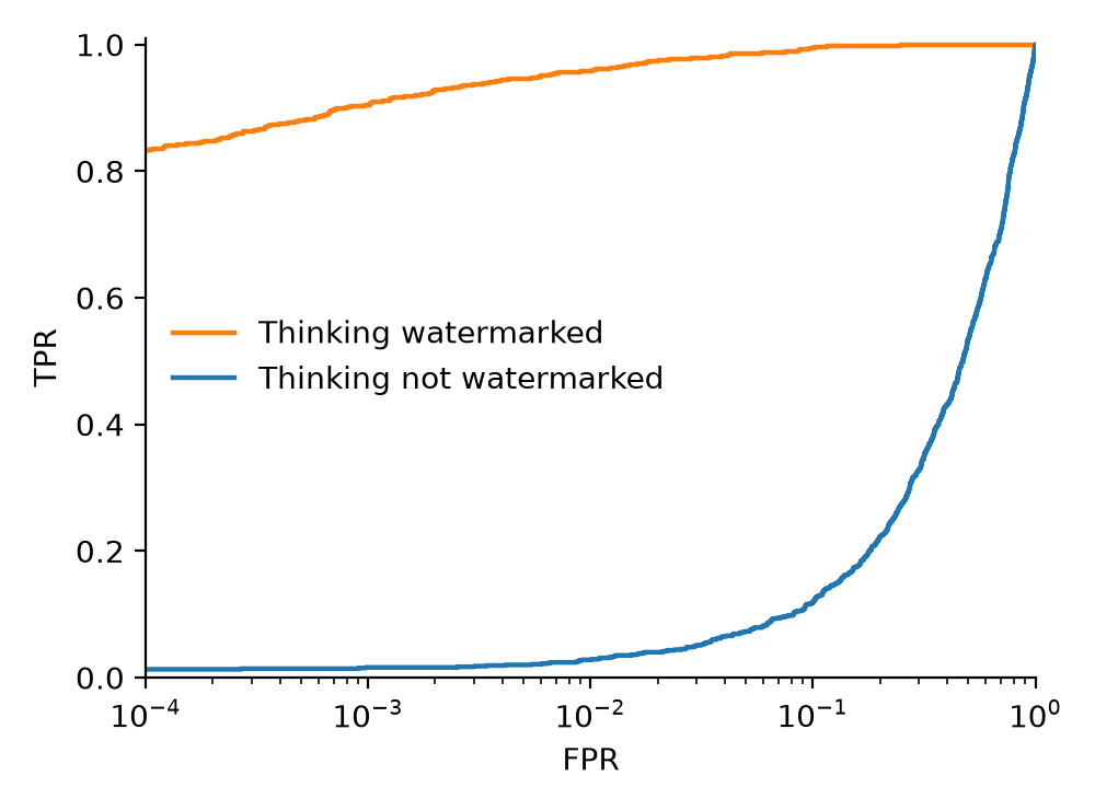
Specifically, we evaluate our attack on Qwen3.8-27B with 1,000 ELI5 prompts and a SynthID watermark with a context of 4 tokens, with final-answer watermarking enabled in both conditions. We only change whether the thinking trace is also watermarked. We use the following prompt:
Answer in 10 sentences exactly this question: {eli5 question}
As we can see in the attached figure, when the thinking is watermarked, we can easily detect the watermark even at low FPRs. However, when the thinking is not watermarked, the watermark is almost undetectable (TPR=FPR).