
Multi-neuron Relaxation Guided Branch-and-bound
Claudio Ferrari, Mark Niklas Müller, Nikola Jovanović
April 21, 2022
This blog post explains the high-level concepts and intuitions behind our most recent neural network verifier MN-BaB. First, we introduce the neural network verification problem. Then, we present the so-called Branch-and-Bound approach for solving it and outline the main ideas behind multi-neuron constraints, before combining the two in our new verifier MN-BaB. We conclude with some experimental results and insights on why using multi-neuron constraints is key for the verification of challenging networks with high natural accuracy.
Neural Network Verification
In a nutshell, the neural network verification problem can be stated as follows:
Given a network and an input, prove that all points in a small region around that input are classified correctly, i.e., that no adversarial example exists.
To formalize this a bit, we consider a network $f: \mathcal{X} \to \mathcal{Y}$, an input region $\mathcal{D} \subseteq \mathcal{X}$, and a linear property $\mathcal{P}\subseteq \mathcal{Y}$ over the output neurons $y\in\mathcal{Y}$, and we try to prove that
\[f(x) \in \mathcal{P}, \forall x \in \mathcal{D}.\]For the sake of explanation, we consider a fully connected $L$-layer network with ReLU activations but note that we can handle all common architectures. We denote the weights and biases of neurons in the $i$-th layer as $W^{(i)}$ and $b^{(i)}$ and define the neural network as
\[f(x) := \hat{z}^{(L)}(x), \qquad \hat{z}^{(i)}(x) := W^{(i)}z^{(i-1)}(x) + b^{(i)}, \qquad z^{(i)}(x) := \max(0, \hat{z}^{(i)}(x)).\]Where $z^{(0)}(x) = x$ denotes the input, $\hat{z}$ are the pre-activation values, and $z$ the post-activation values. For readability, we omit the dependency of intermediate activations on $x$ from here on.
Let $\mathcal{D}$ be an $\ell_\infty$ ball around an input point $x_0$ of radius $\epsilon$: \(\mathcal{D}_\epsilon(x_0) = \left\{ x \in \mathcal{X} \mid \lVert x - x_0\rVert _{\infty} \leq \epsilon \right\}.\)
Since we can encode any linear property over output neurons into an additional affine layer, we can simplify the general formulation of $f(x) \in \mathcal{P}$ to $f(x) > {0}$. Any such property can now be verified by proving that a lower bound to the following optimization problem is greater than $0$:
\[\begin{align*} \min_{x \in \mathcal{D}_\epsilon(x_0)} \qquad &f(x) = \hat{z}^{(L)} \tag{1} \\ s.t. \quad & \hat{z}^{(i)} = W^{(i)}z^{(i-1)} + b^{(i)}\\ & z^{(i)} = \max({0}, \hat{z}^{(i)})\\ \end{align*}\]Background: Branch-and-Bound for Neural Network Verification
Recently, the Branch-and-Bound (BaB) approach, first described for this task in Branch and Bound for Piecewise Linear Neural Network Verification, has been popularized. At a high level, it is based on splitting the hard optimization problem of Eq. 1 into multiple easier subproblems by adding additional constraints until we can show the desired bound of $f(x) > 0$ on them.
The high-level motivation is the following: the optimization problem in Eq. 1 would be efficiently solvable if not for the non-linearity of the ReLU function. Since a ReLU function is piecewise linear and composed of only two linear regions, we can make a case distinction between a single ReLU node being “active” (input $\geq 0$) or inactive (input $< 0$) and prove the property on the resulting cases where the ReLU behaves linearly.
In the limit where all ReLU nodes are split, the verification problem becomes fully linear and can be solved efficiently. However, the number of subproblems to be solved in the resulting Branch-and-Bound tree is exponential in the number of ReLU neurons on which we split. Therefore, splitting all ReLU nodes is computationally intractable for all interesting verification problems. To tackle this problem, we prune this Branch-and-Bound tree using the insight that we do not have to split a subproblem further, once we find a lower bound that is $>0$.
In pseudo-code, the Branch-and-Bound algorithm looks as follows:
    def verify_with_branch_and_bound(network, input_region, output_property) -> bool:
      problem_instance = (input_region, output_property)

      global_lb, global_ub = bound(network, problem_instance)
      unsolved_subproblems = [(global_lb, problem_instance)]

      while global_lb < 0 and global_ub >= 0:
            _, current_subproblem = unsolved_subproblems.pop()
            current_lb, current_ub = bound(network, current_subproblem)

            if current_ub < 0:
              return False
            if current_lb < 0:
              subproblem_left, subproblem_right = branch(current_subproblem)
              unsolved_subproblems.append(subproblem_left, subproblem_right)

            global_lb = min(lb for lb, _ in unsolved_subproblems)
      return global_lb > 0
To define one particular verification method that follows the Branch-and-Bound approach, such as MN-BaB, all we have to do is instantiate the branch() and bound() functions.
Background: Multi-Neuron Constraints
Before we do that, we need to understand multi-neuron constraints (MNCs), the second key building block of MN-BaB.
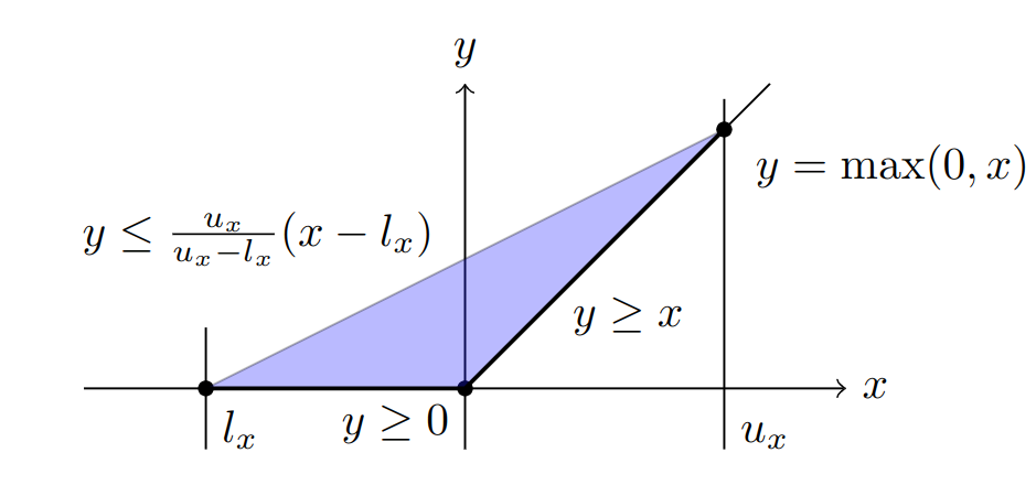
To bound the optimization problem in Eq. 1 efficiently, we want to replace the non-linear constraint $z = \max({0}, \hat{z})$ with its so-called linear relaxation, i.e., a set of linear constraints that is satisfied for all points satisfying the original non-linear constraint. If we consider just a single neuron, the tightest such linear relaxation is the convex hull of the function in its input-output space:
However, considering one neuron at a time comes with a fundamental precision limit, called the (single-neuron) convex relaxation barrier. It has since been shown, that this limit can be overcome by considering multiple neurons jointly, thereby capturing interactions between these neurons and obtaining tighter bounds. We illustrate this improvement, showing a projection of the 4d input-output space of two neurons, below.
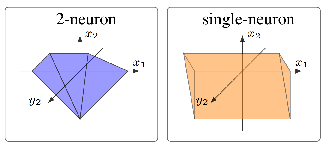
The difference in tightness between the tightest single-neuron, and a multi-neuron relaxation.
We use the efficiently computable multi-neuron constraints from PRIMA, which can be expressed as a conjunction of linear constraints over the joint input-output space.
MN-BaB: Bounding
The goal of the bound() method is to derive a lower bound to Eq. 1 that’s as tight as possible. The tighter it is, the earlier the Branch-and-Bound process can be terminated.
Following previous works, we derive a lower bound of the network’s output as a linear function of the inputs:
\[\min_{x \in \mathcal{D}} f(x) \geq \min_{x \in \mathcal{D}} a_{inp}x + c_{inp}\]There, the minimization over $x \in \mathcal{D}$ has a closed-form solution given by Hölder’s inequality:
\[\min_{x \in \mathcal{D}} a_{inp}x + c^{(0)} \geq a_{inp}x_0 - \lVert a_{inp} \rVert_1 \epsilon + c_{inp}\]To arrive at such a linear lower bound of the output in terms of the input, we start with the trivial lower bound $f(x) \geq z^{(L)}W + b^{(L)}$ and replace $z^{(L)}$ with symbolic, linear bounds depending only on the previous layer’s values $z^{(L-1)}$. We proceed in this manner recursively until we obtain an expression only in terms of the inputs of the network.
These so-called linear relaxations of the different layer types determine the precision of the obtained bounding method. While affine layers (e.g., fully connected, convolutional, avg. pooling, normalization) can be captured exactly, non-linear activation layers remain challenging and their encoding is what differentiates MN-BaB. Most importantly, MN-BaB enforces MNCs in an efficiently optimizable fashion. The full details are given in the paper but are rather technical and notation-heavy, so we will skip them here.
To derive the linear relaxations for activation layers, we need bounds on the inputs of those layers ($l_x$ and $u_x$ in the illustrations). In order to compute these lower and upper bounds on every neuron, we apply the procedure described above to every neuron in the network, starting from the first activation layer.
Note that if those input bounds for a ReLU node are either both negative or both positive, the corresponding activation function becomes linear and we do not have to split this node during the Branch-and-Bound process. We call such nodes “stable” and correspondingly nodes where the input bounds contain zero “unstable”.
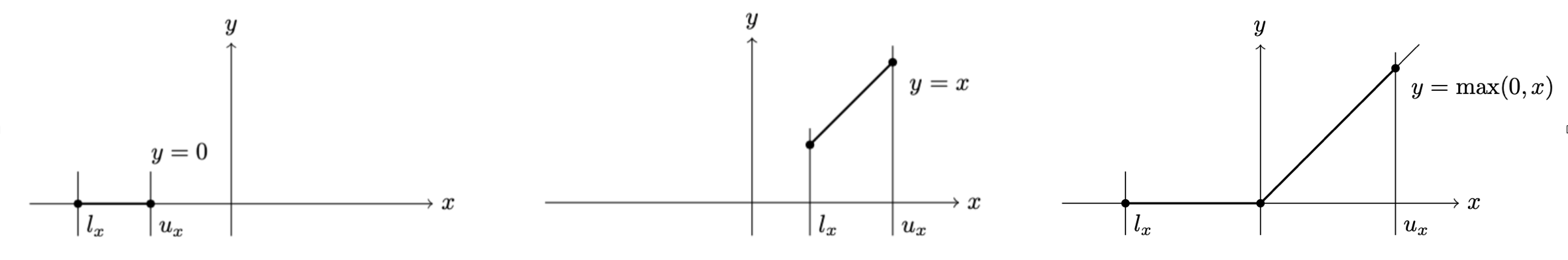
From Left to Right: stable inactive, stable active, unstable.
MN-BaB: Branching
The branch() method takes a problem instance and splits it into two subproblems. This means deciding which unstable ReLU node to split and adding additional constraints to both resulting subproblems enforcing $\hat{z}<0$ or $\hat{z}\geq0$, on the input of the split neuron.
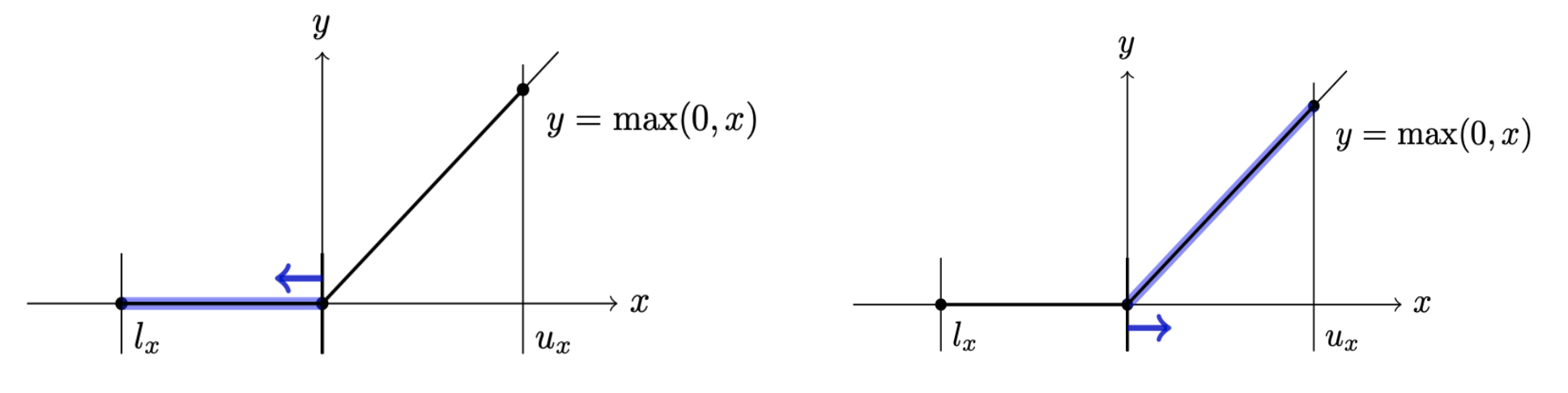
Illustration of the split constraints that are added to the generated subproblems.
The choice of which node to split has a significant impact on how many subproblems we have to consider during the Branch-and-Bound process until we can prove a property. Therefore, we aim to choose a neuron that minimizes the total number of problems we have to consider. To do this, we define a proxy score trying to capture the bound improvement resulting from any particular split. Note that the optimal branching decision depends on the bounding method that is used, as different bounding methods might profit differently from additional constraints resulting from the split.
As our bounding method relies on MNCs, we design a proxy score that is specifically tailored to them, called the Active Constraint Score (ACS). ACS determines the sensitivity of the final optimization objective with respect to the MNCs and then, for each node, computes the cumulative sensitivity of all constraints containing that node. We then split the node with the highest cumulative sensitivity.
We further propose Cost Adjusted Branching (CAB) to scale this branching score by the expected cost of performing a particular split. This cost can differ significantly, as only the intermediate bounds after the split layer have to be recomputed, making splits in later layers computationally cheaper.
Why use multi-neuron constraints?
Using MNCs for bounding, while making the bounds more precise, is computationally costly. The intuitive argument why it still helps verification performance is that the number of subproblems solved during Branch-and-Bound grows exponentially with the depth of the subproblem tree. A more precise bounding method that can verify subproblems earlier (at a smaller depth), can therefore save us exponentially many subproblems that we do not need to solve, which more than compensates for the increased computational cost.
This benefit is more pronounced the larger the considered network and the more dependencies there are between neurons in the same layer. Most established benchmarks (e.g., from VNNComp) are based on very small networks or use training methods designed for ease of verification at the cost of natural accuracy. While this makes their certification tractable, they are less representative of networks used in practice. Therefore, we suggest focusing on larger, more challenging networks with higher natural accuracy (and more intra-layer dependencies) for the evaluation of the next generation of verifiers. There, the benefits of MNCs are particularly pronounced, leading us to believe that they represent a promising direction.
Experiments
We study the effect of MN-BaB’s components in an ablation study on the first 100 test images of the CIFAR-10 dataset. We aim to prove that there is no adversarial example within an $\ell_\infty$ ball of radius $\epsilon=1/255$ and report the number of verified samples (within a timeout of 600 seconds) and the corresponding average runtime. We consider two networks of identical architecture that only differ in the strength of their adversarial training method. ResNet6-A is weakly regularized while ResNet6-B is more strongly regularized, i.e. employs stronger adversarial training.
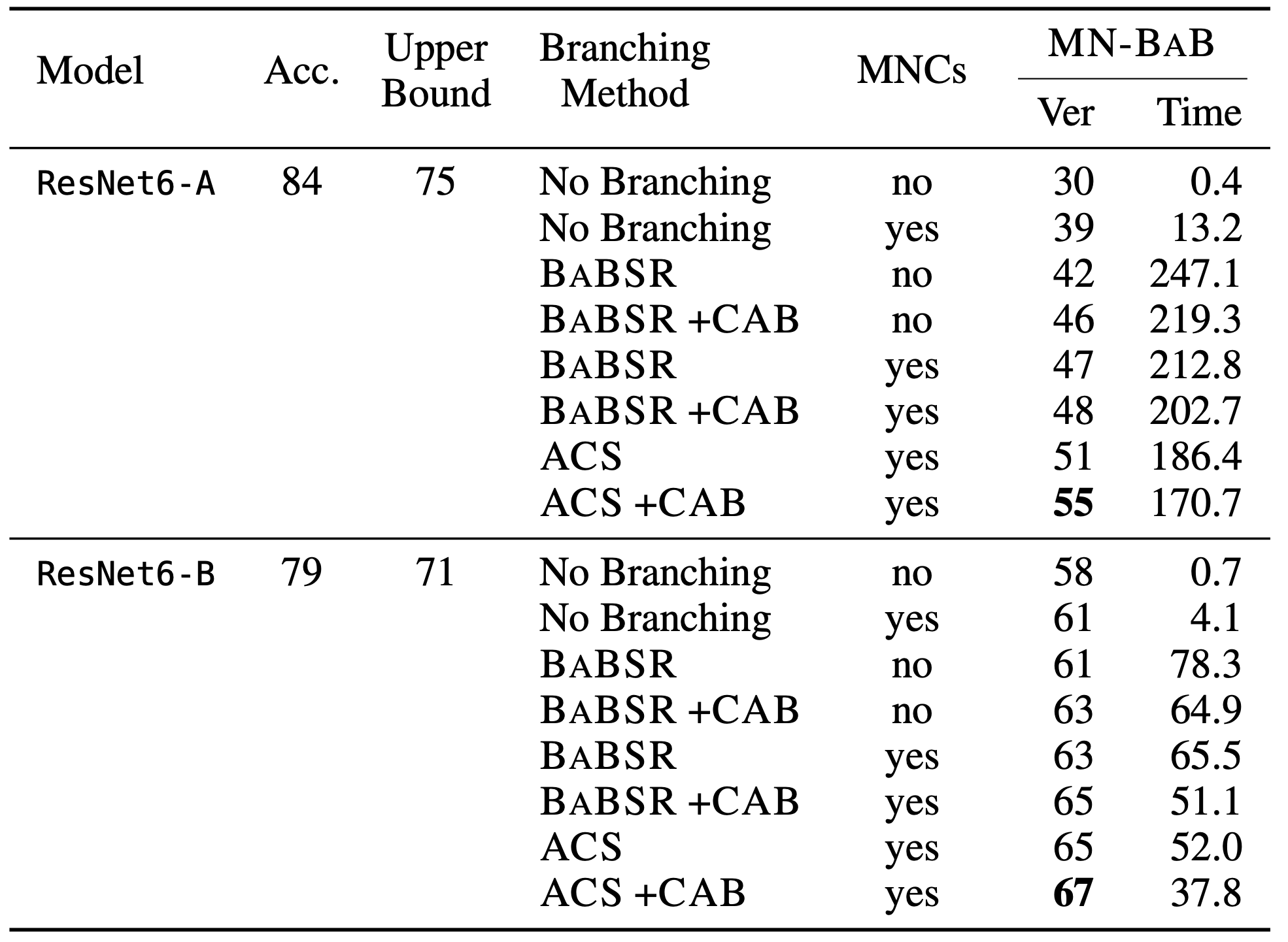
Evaluating the effect of MNCs, Active Constraint Score (ACS) branching, and Cost Adjusted Branching (CAB) on MN-BaB. BaBSR is another branching method that is used as a baseline.
As expected, we see that both MNCs and Active Constraint Score branching are much more effective on the weakly regularized ResNet6-A. There, we verify 31% more samples while being around 31% faster, while on ResNet6-B we only verify 10% more samples.
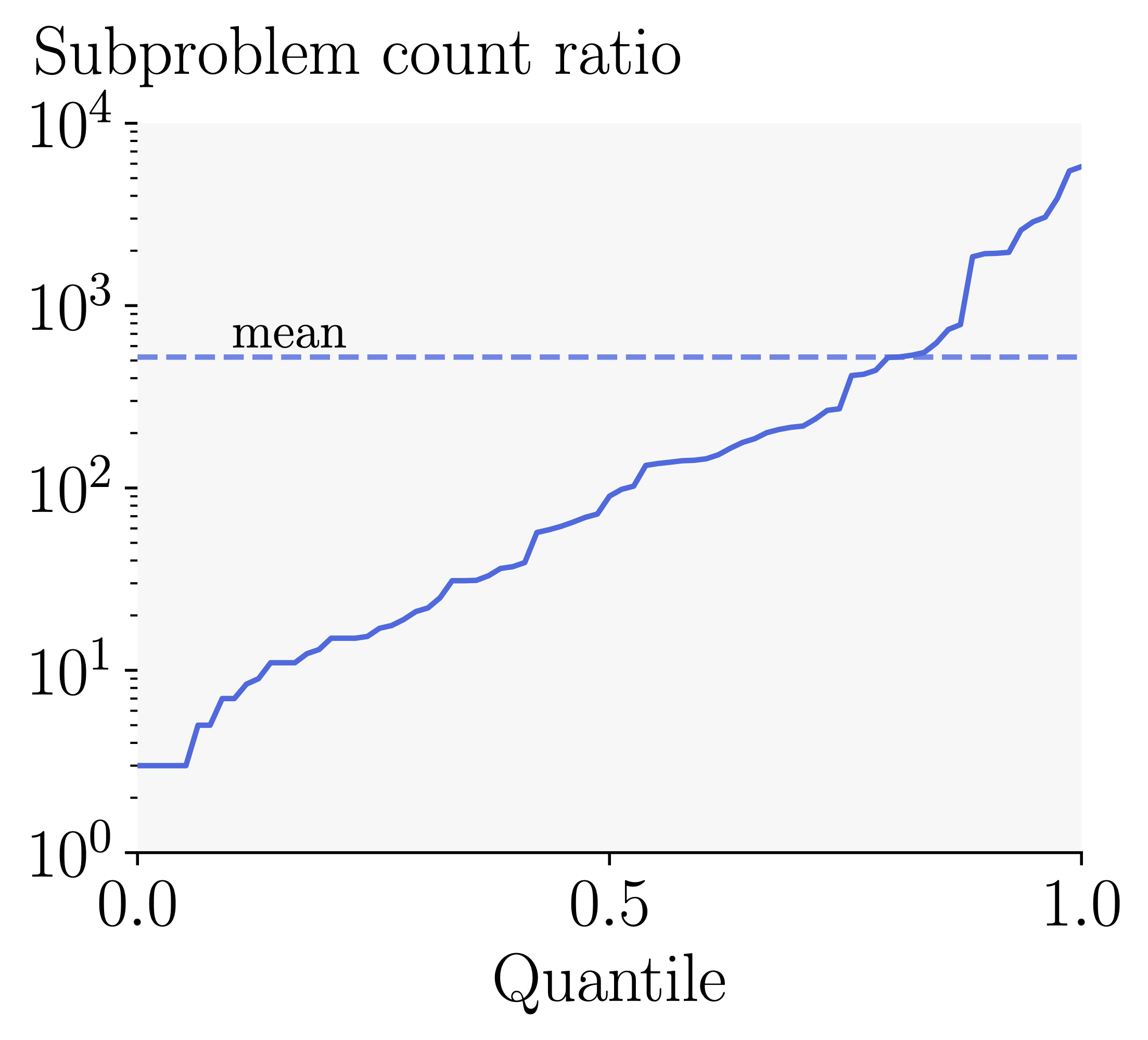
As a more fine-grained measure of performance, we analyze the ratio of runtimes and number of subproblems required for verification on a per-property level on ResNet6-A.
Effectiveness of Multi-Neuron Constraints: We plot the ratio of the number of subproblems required to prove a property during Branch-and-Bound without vs. with MNCs. Using MNCs reduces the number of subproblems by two orders of magnitude on average.
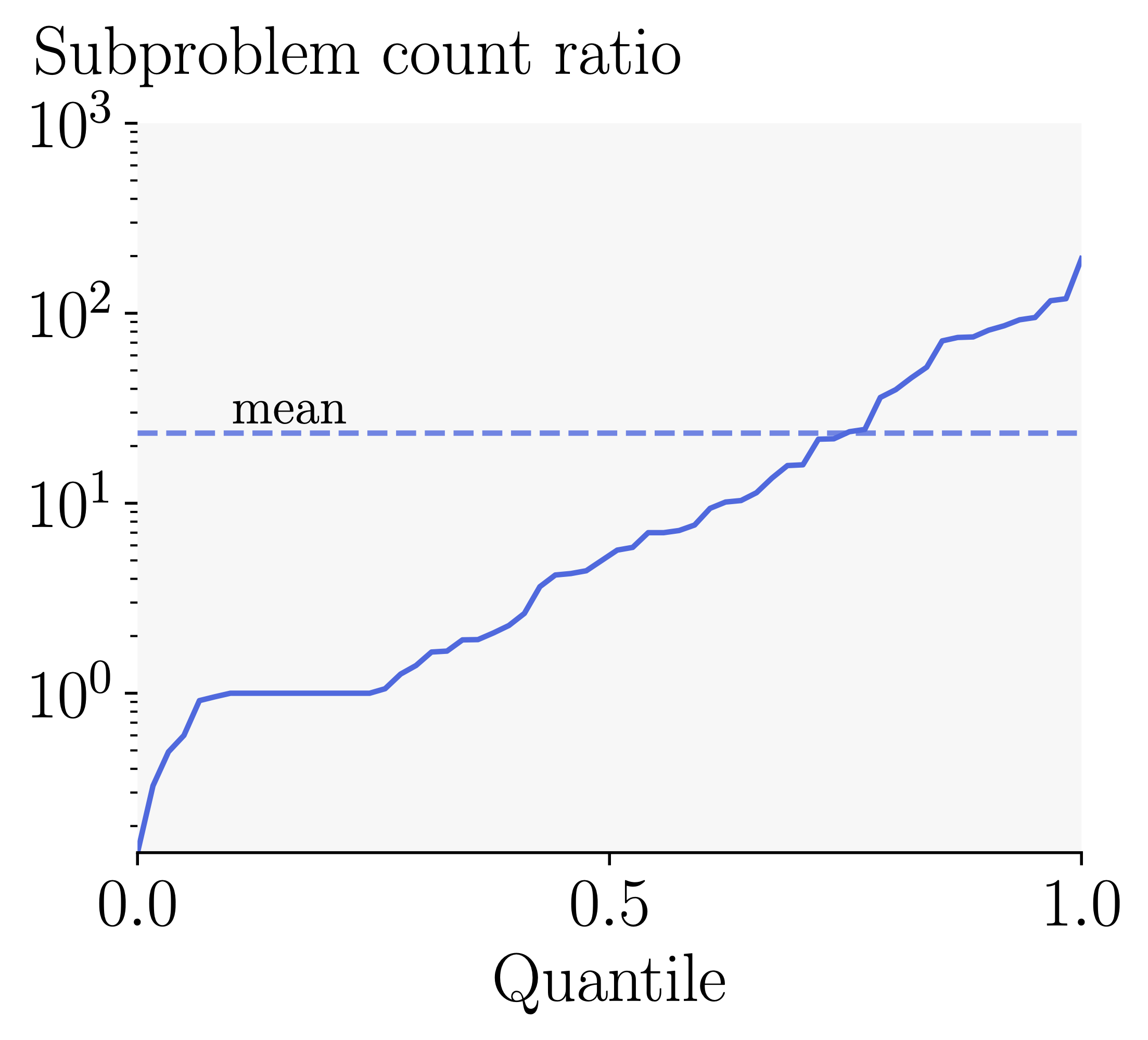
Effectiveness of Active Constraint Score Branching: We plot the ratio of the number of subproblems solved during Branch-and-Bound with BaBSR vs. ACS. Using ACS reduces the number of subproblems by an additional order of magnitude.
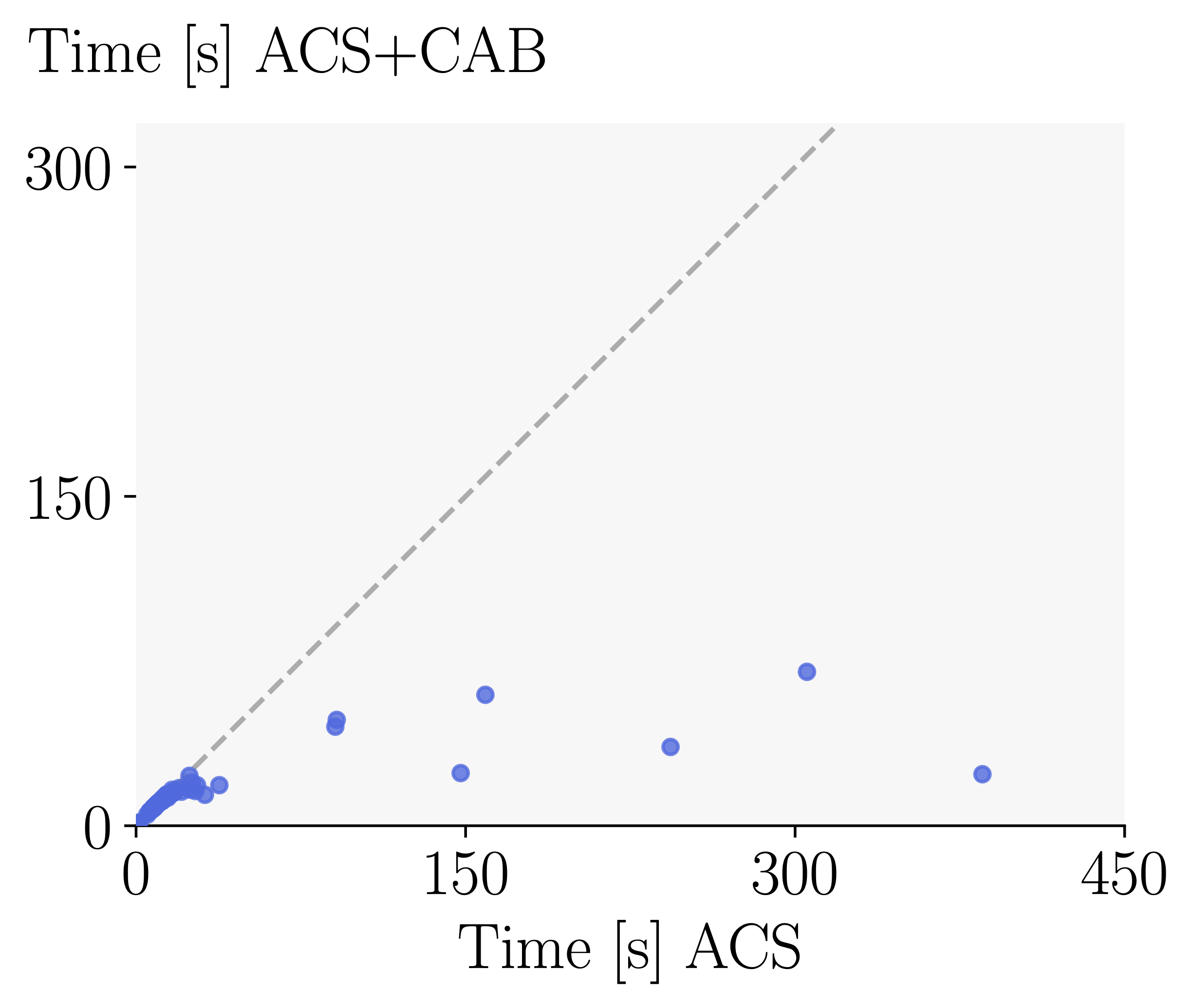
Effectiveness of Cost Adjusted Branching: Finally, we investigate the effect of Cost Adjusted Branching on mean verification time with ACS. Using Cost Adjusted Branching further reduces the verification time by 50%. It is particularly effective in combination with the ACS scores and multi-neuron constraints, where bounding costs vary more significantly.
Recap
MN-BaB combines precise multi-neuron constraints with the Branch-and-Bound paradigm and an efficient GPU-based implementation to become a new state-of-the-art verifier, especially for less regularized networks. For a full breakdown of all technical details and detailed experimental evaluations, we recommend reading our paper. If you want to play around with MN-BaB yourself, please check out our code.